Computer Vision - Experiment 12 - Discrete Fourier Transform Experiment

Experimental objectives and requirements

  Understand the basic principle of Fourier transform; master the code writing method to implement Fourier transform.

Experiment content

   (i) New project.

   (ii) Configure OpenCV in VS2015.

   (iii) Read the original image in grayscale mode and display it;

   (iv) Write code to implement the Fourier transform;

   (v) Display the Fourier transform effect graph.

Experimental apparatus, equipment

  A computer with Windows 7 operating system and Visual Studio 2015 installed

Experimental principle

   (i) Discrete Fourier transform (DFT), which is the Fourier transform in both the time and frequency domains in a discrete form, transforms the sampling of the time-domain signal into sampling in the frequency domain of the discrete-time Fourier transform. Formally, the sequences at both ends of the transform (in the time and frequency domains) are finite-length, while in practice both sets of sequences should be considered as principal value sequences of discrete periodic signals. Even if a DFT is done for a finite-length discrete signal, it should be transformed again after it has been extended periodically to become a periodic signal. In practical applications, the fast Fourier transform is usually used to compute the DFT efficiently.

   (ii) Inside the frequency domain, for an image, places with intense changes in brightness or grayscale correspond to high-frequency components, such as edge and texture information; places with little change in brightness or grayscale correspond to low-frequency components. If the image is subjected to noise that happens to lie within a specific “frequency” range, the original image can be recovered by a filter. Fourier transform can be used in image processing for image enhancement and image denoising, image segmentation and edge detection, image feature extraction, image compression, etc.

Experimental steps

   (i) Create Visual Studio 2015 console program;

   (ii) Configure OpenCV in Visual Studio 2015;

   (iii) Reading the original image in grayscale mode and displaying it;

   (iv) Extend the input image to the optimal size, with borders supplemented by 0;

   (v) Allocate storage space for the results of the Fourier transform (real and imaginary parts);

   (vi) Performing the discrete Fourier transform;

   (vii) Convert the complex numbers into magnitudes;

   (viii) Performing logarithmic scale scaling;

   (ix) shear and redistribute the magnitude map quadrant;

   (x) Normalization, transforming the matrix into a visual image format using floating point values between 0 and 1;

   (xi) Display the Fourier transform effect map.

Experimental notes

   (i) The method of configuring OpenCV in VS after completing the installation of OpenCV;

   (ii) The functions and usage of the dft function;

   (iii) The method of clipping and redistributing magnitude map quadrants;

   (iv) The function and usage of the normalize function.

Experimental results

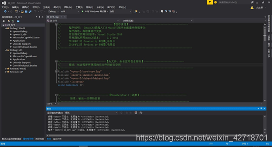
   (i) Experimental code

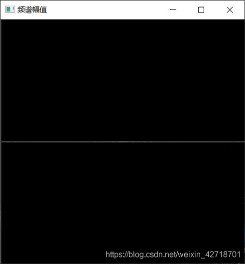
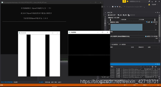
 1
 2
 3
 4
 5
 6
 7
 8
 9
10
11
12
13
14
15
16
17
18
19
20
21
22
23
24
25
26
27
28
29
30
31
32
33
34
35
36
37
38
39
40
41
42
43
44
45
46
47
48
49
50
51
52
53
54
55
56
57
58
59
60
61
62
63
64
65
66
67
68
69
70
71
72
73
74
75
76
77
78
79
80
81
82
83
84
85
86
87
88
89
90
91
92
93
94
95

//-----------------------【头文件、命名空间包含部分】-----------------------------
//		描述：包含程序所使用的头文件和命名空间
//---------------------------------------------------------------------------------
#include "opencv2/core/core.hpp"
#include "opencv2/imgproc/imgproc.hpp"
#include "opencv2/highgui/highgui.hpp"
#include <iostream>
using namespace cv;


//-----------------------------------【ShowHelpText( )函数】------------------------
//		 描述：输出一些帮助信息
//----------------------------------------------------------------------------------
void ShowHelpText()
{
	//输出欢迎信息和OpenCV版本
	printf("\n\n\t\t\t非常感谢购买《OpenCV3编程入门》一书！\n");
	printf("\n\n\t\t\t此为本书OpenCV3版的第28个配套示例程序\n");
	printf("\n\n\t\t\t   当前使用的OpenCV版本为：" CV_VERSION );
	printf("\n\n  ----------------------------------------------------------------------------\n");
}



//-------------------------------【main( )函数】-----------------------------------------
//          描述：控制台应用程序的入口函数，我们的程序从这里开始执行
//-------------------------------------------------------------------------------------
int main( )
{

	//【1】以灰度模式读取原始图像并显示
	Mat srcImage = imread("feng.png", 0);
	if(!srcImage.data ) { printf("读取图片错误，请确定目录下是否有imread函数指定图片存在~！ \n"); return false; } 
	imshow("原始图像" , srcImage);   

	ShowHelpText();

	//【2】将输入图像延扩到最佳的尺寸，边界用0补充
	int m = getOptimalDFTSize( srcImage.rows );
	int n = getOptimalDFTSize( srcImage.cols ); 
	//将添加的像素初始化为0.
	Mat padded;  
	copyMakeBorder(srcImage, padded, 0, m - srcImage.rows, 0, n - srcImage.cols, BORDER_CONSTANT, Scalar::all(0));

	//【3】为傅立叶变换的结果(实部和虚部)分配存储空间。
	//将planes数组组合合并成一个多通道的数组complexI
	Mat planes[] = {Mat_<float>(padded), Mat::zeros(padded.size(), CV_32F)};
	Mat complexI;
	merge(planes, 2, complexI);         

	//【4】进行就地离散傅里叶变换
	dft(complexI, complexI);           

	//【5】将复数转换为幅值，即=> log(1 + sqrt(Re(DFT(I))^2 + Im(DFT(I))^2))
	split(complexI, planes); // 将多通道数组complexI分离成几个单通道数组，planes[0] = Re(DFT(I), planes[1] = Im(DFT(I))
	//void magnitude(InputArray x, InputArray y, OutputArray magnitude);
	magnitude(planes[0], planes[1], planes[0]);// planes[0] = magnitude  
	Mat magnitudeImage = planes[0];

	//【6】进行对数尺度(logarithmic scale)缩放
	magnitudeImage += Scalar::all(1);
	log(magnitudeImage, magnitudeImage);//求自然对数

	//【7】剪切和重分布幅度图象限
	//若有奇数行或奇数列，进行频谱裁剪      
	magnitudeImage = magnitudeImage(Rect(0, 0, magnitudeImage.cols & -2, magnitudeImage.rows & -2));
	//重新排列傅立叶图像中的象限，使得原点位于图像中心  
	int cx = magnitudeImage.cols/2;
	int cy = magnitudeImage.rows/2;
	Mat q0(magnitudeImage, Rect(0, 0, cx, cy));   // ROI区域的左上
	Mat q1(magnitudeImage, Rect(cx, 0, cx, cy));  // ROI区域的右上
	Mat q2(magnitudeImage, Rect(0, cy, cx, cy));  // ROI区域的左下
	Mat q3(magnitudeImage, Rect(cx, cy, cx, cy)); // ROI区域的右下
	//交换象限（左上与右下进行交换）
	Mat tmp;                           
	q0.copyTo(tmp);
	q3.copyTo(q0);
	tmp.copyTo(q3);
	//交换象限（右上与左下进行交换）
	q1.copyTo(tmp);                 
	q2.copyTo(q1);
	tmp.copyTo(q2);

	//【8】归一化，用0到1之间的浮点值将矩阵变换为可视的图像格式
	//此句代码的OpenCV2版为：
	//normalize(magnitudeImage, magnitudeImage, 0, 1, CV_MINMAX); 
	//此句代码的OpenCV3版为:
	normalize(magnitudeImage, magnitudeImage, 0, 1, NORM_MINMAX); 

	//【9】显示效果图
	imshow("频谱幅值", magnitudeImage);    
	waitKey();

	return 0;
}

   (ii) Show results

Experiment summary

  The main content of this experiment is to understand the basic principle of Fourier transform; to master the code writing method to implement Fourier transform. Create a new project, configure OpenCV in VS2015; read the original image in grayscale mode and display it; write code to realize the Fourier transform; display the Fourier transform effect graph.