Machine Learning - Linear regression experiments
Learning linear regression with scikit-learn and pandas
1. Get the data, define the problem
We ran linear regression with publicly available machine learning data from UCI University.
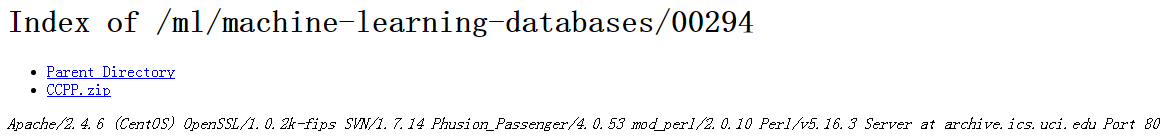
The data can be downloaded here:https://archive.ics.uci.edu/ml/datasets/combined+cycle+power+plant The downloaded data can be found as a compressed file, after decompression there is an xlsx file, open it with excel, save it as a csv format, and later use this csv format file to run linear regression.
This is a cyclic generation field data with 9568 sample data, each with 5 columns: $AT$ (Temperature), $V$ (Pressure), $AP$ (Humidity), $RH$ (Pressure), $PE$ (Output power). We don’t need to get hung up on the exact meaning of each item.
Our problem is to obtain a linear relationship corresponding to PE as the sample output and $AT, V, AP, RH$ which are the four sample features, and machine learning aims to obtain a linear regression model, i.e:
$$
PE= \theta_0+ \theta_1 \times AT+ \theta_2 \times V + \theta_3 \times AP + \theta_4 \times RH
$$
And all that needs to be learned are the five parameters $\theta_0, \theta_1, \theta_2, \theta_3, \theta_4$.
2. Organizing data
Opening this csv reveals that the data are already organized and there are no illegal data, so no preprocessing is needed. However, the data are not normalized, i.e., they are converted to a mean 0, variance 1 format. (scikit-learn will automatically normalize the data for us in linear regression).
Open JupyterNotebook, import the dataset in the Home page, and don’t forget to upload it. Then create a new Python3 note.
 1
 2
 3
 4
 5
 6
 7
 8
 9
10
11
12
13
14
15
16
17
18
19
20
21
22
23
24
25
26
27
|
#Importing related class libraries
import matplotlib.pyplot as plt #Drawing Gallery
#Set up illustrations so that they are visible in Notepad
%matplotlib inline
import numpy as np
import pandas as pd
from sklearn import datasets, linear_model
#Read data with pandas
data = pd.read_csv('ccpp.csv')
data.describe()
#View the first 5 rows of data
data.head()
#View the last 5 rows of the data
data.tail()
#View the dimensions of the data
data.shape
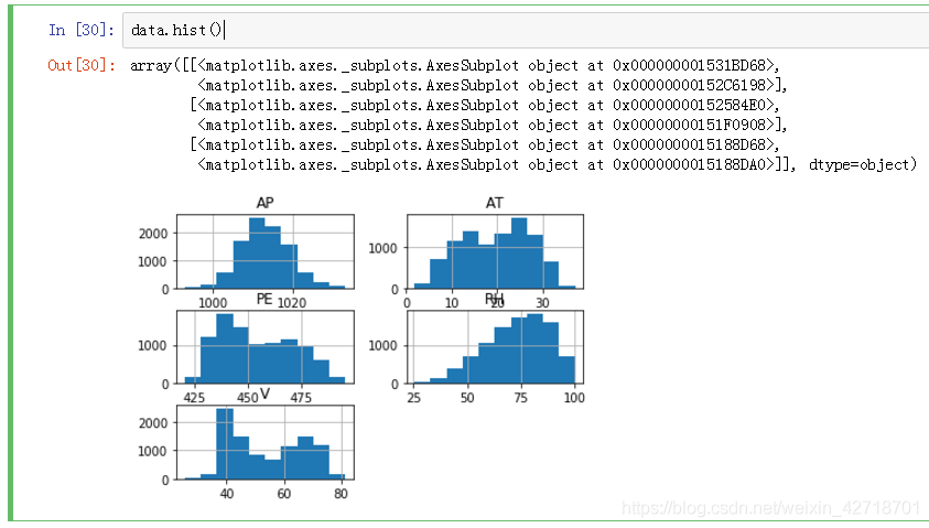
#Data visualization, histogram display
data.hist()
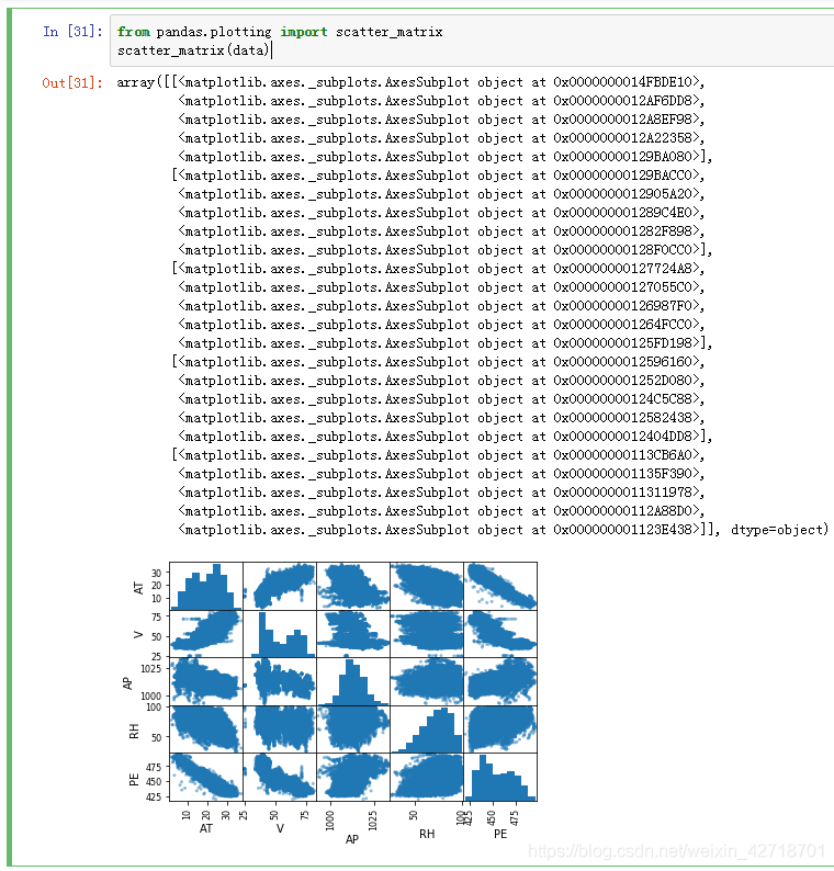
#Scatter matrix
from pandas.plotting import scatter_matrix
scatter_matrix(data)
|
3. Prepare data
The dataset has 9568 samples with 5 cases each.
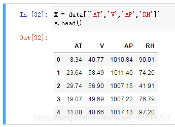
In the following, we start preparing the sample features $X$, and we use the four columns $AT, V, AP$ and $RH$ as sample features.
1
2
|
X = data[['AT','V','AP','RH']]
X.head()
|
Prepare the sample output $y$, and we use $PE$ as the sample output.
1
2
|
y = data[['PE']]
y.head()
|
Divide the training and test sets to divide the combination of $X$ and $y$ samples into two parts, one for the training set and one for the test set. Use the train_test_split function, official documentation at
https://scikit-learn.org/stable/modules/generated/sklearn.model_selection.train_test_split.html#sklearn.model_selection.train_test_split
1
2
|
from sklearn.model_selection import train_test_split
X_train,X_test,y_train,y_test = train_test_split(X, y, random_state=1)
|
Parameters:
test_size: the size of the test set. If floating-point, it is between 0.0 and 1.0 and represents the proportion of the test set; if integer, it is the absolute number of test set samples; if not, it is the complement of the training set. By default, the value is 0.25. In addition, it is version dependent.
train_size: the size of the training set. If floating-point, it is between 0.0 and 1.0 and represents the proportion of the training set; if integer, it is the absolute number of training set samples; if not, it is the complement of the test set.
random_state: specifies the random method. An integer or randomState instance, or None. if integer, it specifies the seed of the random number generator; if RandomState instance, it specifies the random number generator; if None, it uses the default random number generator and chooses a random seed.
shuffle: Boolean value. Whether to reorganize the data before splitting. If shuffle=False, then stratify must be None.
stratify: array-likeorNone. if not None, then the dataset is split in a hierarchical way and this is used as the class label.
Return value: the splitting of the resulting train and test datasets.
1
2
3
4
5
|
#Looking at the dimensions of the training and test sets, we can see that 75% of the sample data is used as the training set and 25% of the samples are used as the test set.
print(X_train.shape)
print(y_train.shape)
print(X_test.shape)
print(y_test.shape)
|
4. Training data
A linear model with scikit-learn is used to fit our problem.
1
2
3
|
fromsklearn.linear_modelimportLinearRegression#Ordinary linear regression model, using least squares to fit the data
linreg = LinearRegression()
linreg.fit(X_train,y_train)
|
The linear regression fit function is used to fit the input and output data and is called in the form of $model.fit(X,y,sample_weight=None):
•X:X is the training vector;
•y:y is the target vector relative to X;
•sample_weight:Array of weights assigned to each sample, generally not needed and can be omitted.
Note: $X$, $y$ and the values returned by model.fit() are 2-D arrays, e.g., $a=[[0]]$
1
2
3
|
#After the fit is completed, the resulting model parameters are viewed:
print(linreg.intercept_)
print(linreg.coef_)
|
This gives us the values of the five parameters that need to be found inside the linear regression model.
5. Model Evaluation
After the model is trained, we need to evaluate how good or bad the model is. For linear regression, we generally use Mean Squared Error (MSE) or Root Mean Squared Error (RMSE) on the test set to evaluate how good or bad the model is. If we get different parameters by other methods and need to choose a model, we use the model parameters with small MSE.
1
2
3
4
5
6
7
|
#Model Fitting Test Set
y_pred = linreg.predict(X_test)
from sklearn import metrics
#Calculating MSE with scikit-learn
print("MSE:",metrics.mean_squared_error(y_test,y_pred))
#Calculating RMSE with scikit-learn
print("RMSE:",np.sqrt(metrics.mean_squared_error(y_test,y_pred)))
|
Experiment with different linear models for training
Add the regularization term, Ridge regression model,L2 parametric call Ridge function Students manually adjust the value of alpha and observe the change in results. Think: How does the alpha value relate to over-fitting and under-fitting?
1
2
3
4
5
|
from sklearn.linear_model import Ridge
rdg = Ridge(alpha=10000,fit_intercept=True)
rdg.fit(X_train,y_train)
print(rdg.intercept_)
print(rdg.coef_)
|
#Model Fitting Test Set
1
2
3
4
5
6
|
y_pred = rdg.predict(X_test)
from sklearn import metrics
#Calculating MSE with scikit-learn
print("MSE:",metrics.mean_squared_error(y_test,y_pred))
#Calculating RMSE with scikit-learn
print("RMSE:",np.sqrt(metrics.mean_squared_error(y_test,y_pred)))
|
Lasso regression model with L1 paradigm
Calling the LASSO function
1
2
3
4
5
|
from sklearn.linear_model import Lasso
las = Lasso(alpha=0.1)
las.fit(X_train,y_train)
print(las.intercept_)
print(las.coef_)
|
#Model Fitting Test Set
1
2
3
4
5
6
7
|
y_pred = las.predict(X_test)
from sklearn import metrics
#Calculating MSE with scikit-learn
print("MSE:",metrics.mean_squared_error(y_test,y_pred))
#Calculating RMSE with scikit-learn
print("RMSE:",np.sqrt(metrics.mean_squared_error(y_test,y_pred)))
print("Number of iterations:",las.n_iter_)
|
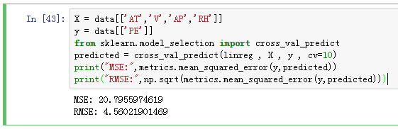
Cross-validation
We can continuously optimize the model by cross-validation using 10-fold cross-validation, i.e., the cv parameter in cross_val_predict is 10:
1
2
3
4
5
6
7
8
|
X = data[['AT','V','AP','RH']]
y = data[['PE']]
from sklearn.model_selection import cross_val_predict
predicted=cross_val_predict(linreg,X,y,cv=10)
#Calculating MSE with scikit-learn
print("MSE:",metrics.mean_squared_error(y,predicted))
#Calculating RMSE with scikit-learn
print("RMSE:",np.sqrt(metrics.mean_squared_error(y,predicted)))
|
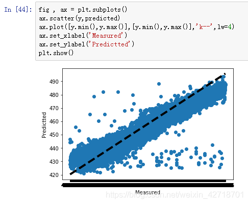
6. Graphical observation of the results
Draw a graph to observe the relationship between the true and predicted values. The closer the point is to the middle line y=x, the lower the predicted loss is represented.
1
2
3
4
5
6
7
|
fig,ax = plt.subplots()
ax.scatter(y,predicted)
ax.plot([y.min(),y.max()],[y.min(),y.max()],'k--',lw=4)
#Try to change k-- to r--, r- and observe the line pattern. To see the details of a function, use the help() function.
ax.set_xlabel('Measured')
ax.set_ylabel('Predicted')
plt.show()
|
7. python program full source code
 1
 2
 3
 4
 5
 6
 7
 8
 9
10
11
12
13
14
15
16
17
18
19
20
21
22
23
24
25
26
27
28
29
30
31
32
33
34
35
36
37
38
39
40
41
42
43
44
45
46
47
48
49
50
51
52
53
54
55
56
57
58
59
60
61
62
63
64
65
66
67
68
69
70
71
72
73
74
75
76
77
78
79
80
81
82
83
|
import matplotlib.pyplot as plt
%matplotlib inline
import numpy as np
import pandas as pd
from sklearn import datasets , linear_model

data = pd.read_csv('ccpp.csv')

data.describe()

data.head()

data.tail()

data.shape

data.hist()

from pandas.plotting import scatter_matrix
scatter_matrix(data)

X = data[['AT','V','AP','RH']]
X.head()

y = data[['PE']]
y.head()

from sklearn.model_selection import train_test_split
X_train , X_test , y_train , y_test = train_test_split(X , y , random_state=1)

print (X_train.shape)
print (y_train.shape)
print (X_test.shape)
print (y_test.shape)

from sklearn.linear_model import LinearRegression
linreg = LinearRegression()
linreg.fit(X_train,y_train)

print(linreg.intercept_)
print(linreg.coef_)

y_pred = linreg.predict(X_test)
from sklearn import metrics
print("MSE:",metrics.mean_squared_error(y_test,y_pred))
print("RMSE:",np.sqrt(metrics.mean_squared_error(y_test,y_pred)))

from sklearn.linear_model import Ridge
rdg = Ridge(alpha=8000,fit_intercept=True)
rdg.fit(X_train,y_train)
print(rdg.intercept_)
print(rdg.coef_)

y_pred = rdg.predict(X_test)
from sklearn import metrics
print("MSE:",metrics.mean_squared_error(y_test,y_pred))
print("RMSE:",np.sqrt(metrics.mean_squared_error(y_test,y_pred)))

from sklearn.linear_model import Lasso
las = Lasso(alpha = 0.1)
las.fit(X_train,y_train)
print (las.intercept_)
print (las.coef_)

y_pred = las.predict(X_test)
from sklearn import metrics
print("MSE:",metrics.mean_squared_error(y_test,y_pred))
print("RMSE:",np.sqrt(metrics.mean_squared_error(y_test,y_pred)))
print("迭代次数:",las.n_iter_)

X = data[['AT','V','AP','RH']]
y = data[['PE']]
from sklearn.model_selection import cross_val_predict
predicted = cross_val_predict(linreg , X , y , cv=10)
print("MSE:",metrics.mean_squared_error(y,predicted))
print("RMSE:",np.sqrt(metrics.mean_squared_error(y,predicted)))

fig , ax = plt.subplots()
ax.scatter(y,predicted)
ax.plot([y.min(),y.max()],[y.min(),y.max()],'k--',lw=4)
ax.set_xlabel('Measured')
ax.set_ylabel('Predictted')
plt.show()
|